Hi all. There’s been lots of discussion about improving TVM documentation. I noticed that there isn’t much documentation for the InferBound pass, but I think it’s an interesting part of the code, that’s fundamental to understanding how lowering works in TVM. After all, InferBound is essential to determining loop extents, and buffer sizes.
So I decided to write documentation for the InferBound pass, both to clarify my own understanding, and to help others gain a deeper understanding of this pass too.
I want to contribute this documentation to the developer docs, but before opening an issue/PR I’d like to solicite feedback from the community. I very much appreciate the time anyone takes to read the documentation below, and provide comments.
InferBound Overview
The InferBound pass is run after normalize, and before ScheduleOps [build_module.py:308]. The main job of InferBound is to create the bounds map, which specifies a Range for each IterVar in the program. These bounds are then passed to ScheduleOps, where they are used to set the extents of For loops [MakeLoopNest], and to set the sizes of allocated buffers [BuildRealize], among other uses.
The output of InferBound is a map from IterVar to Range:
Map<IterVar, Range> InferBound(const Schedule& sch);
Therefore, let’s review the Range and IterVar classes:
namespace HalideIR {
namespace IR {
	class RangeNode : public Node {
	public:
		Expr min;
		Expr extent;
		// remainder ommitted
	};
	}}
namespace tvm {
	class IterVarNode : public Node {
	public:
		Range dom;
		Var var;
		// remainder ommitted
	};
}
Note that IterVarNode also contains a Range ‘dom’. This dom may or may not have a meaningful value, depending on when the IterVar was created. For example, when tvm.compute is called, an IterVar is created for each axis and reduce axis, with dom’s equal to the shape supplied in the call to tvm.compute.
On the other hand, when tvm.split is called, IterVars are created for the inner and outer axes, but these IterVars are not given a meaningful ‘dom’ value.
In any case, the ‘dom’ member of an IterVar is never modified during InferBound. However, keep in mind that the ‘dom’ member of an IterVar is sometimes used as default value for the Ranges InferBound computes.
We next review some TVM codebase concepts that are required to understand the InferBound pass.
Recall that InferBound takes one argument, a Schedule. This schedule object, and its members, contains all information about the program being compiled.
A TVM schedule is composed of Stages. Each stage has exactly one Operation, e.g., a ComputeOp or a TensorComputeOp. Each operation has a list of root_iter_vars, which in the case of ComputeOp, are composed of the axis IterVars and the reduce axis IterVars. Each operation can also contain many other IterVars, but all of them are related by the operations’s list of IterVarRelations. Each IterVarRelation represents either a split, compute_at (rebase) or fuse in the schedule. For example, in the case of split, the IterVarRelation specifies the parent IterVar that was split, and the two children IterVars: inner and outer.
namespace tvm {
	class ScheduleNode : public Node {
	public:
		Array<Operation> outputs;
		Array<Stage> stages;
		Map<Operation, Stage> stage_map;
		// remainder ommitted
	};

	class StageNode : public Node {
	public:
		Operation op;
		Operation origin_op;
		Array<IterVar> all_iter_vars;
		Array<IterVar> leaf_iter_vars;
		Array<IterVarRelation> relations;
		// remainder ommitted
	};

	class OperationNode : public Node {
	public:
		virtual Array<IterVar> root_iter_vars();
		virtual Array<Tensor> InputTensors();
		// remainder ommitted
	};

	class ComputeOpNode : public OperationNode {
	public:
		Array<IterVar> axis;
		Array<IterVar> reduce_axis;
		Array<Expr> body;
		Array<IterVar> root_iter_vars();
		// remainder ommitted
	};
}
Tensors haven’t been mentioned yet, but in the context of TVM, a Tensor represents output of an operation.
class TensorNode : public Node {
public:
	// The source operation, can be None
	// This Tensor is output by this op
	Operation op;
	// The output index from the source operation
	int value_index;
};
In the Operation class declaration above, we can see that each operation also has a list of InputTensors. Thus the stages of the schedule form a DAG, where each stage is a node in the graph. There is an edge in the graph from Stage A to Stage B, if the operation of Stage B has an input tensor whose source operation is the op of Stage A. Put simply, there is an edge from A to B, if B consumes a tensor produced by A. See the diagram below. This graph is created at the beginning of InferBound, by a call to CreateReadGraph.
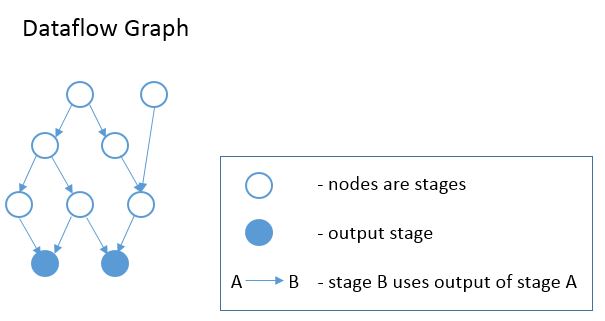
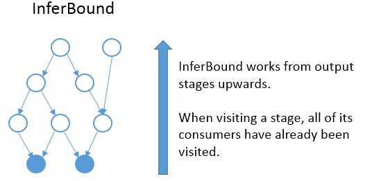
InferBound makes one pass through the graph, visiting each stage exactly once. InferBound starts from the output stages (i.e., the solid blue nodes in the graph above), and moves upwards (in the opposite direction of the edges). Therefore, when InferBound visits a stage, each of its consumer stages has already been visited.
The InferBound pass is shown in the following pseudo-code:
Map<IterVar, Range> InferBound(const Schedule& sch) {
	Array<Operation> outputs = sch->get_outputs();
	G = CreateGraph(outputs);
	stage_list = sch->get_ordered_stages(G);
	Map<IterVar, Range> rmap;
	for (Stage s in stage_list) {
		InferRootBound(s, &rmap);
		PassDownDomain(s, &rmap);
	}
	return rmap;
}
The InferBound pass has two interesting properties that are not immediately obvious:
- After InferBound visits a stage, the ranges of all IterVars in the stage will be set in rmap.
- The Range of each IterVar is only set once in rmap, and then never changed.
So it remains to explain what InferBound does when it visits a stage. As can be seen in the pseudo-code above, InferBound calls two functions on each stage: InferRootBound, and PassDownDomain. The purpose of InferRootBound is to set the Range (in rmap) of each root_iter_var of the stage. (Note: InferRootBound does not set the Range of any other IterVar, only those belonging to root_iter_vars). The purpose of PassDownDomain is to propagate this information to the rest of the stage’s IterVars. When PassDownDomain returns, all IterVars of the stage have known Ranges in rmap.
The remainder of the document dives into the details of InferRootBound and PassDownDomain.
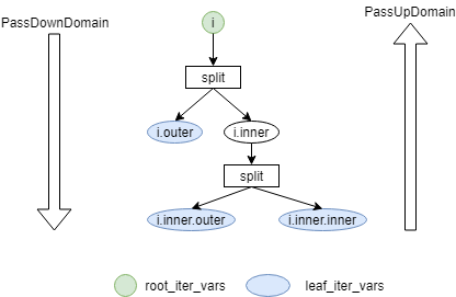
IterVar Hyper-graph
The InferBound pass traverses the stage graph, as described above. However, within each stage is another graph, whose nodes are IterVars. InferRootBound and PassDownDomain perform message-passing on these IterVar graphs.
Recall that all IterVars of the stage are related by IterVarRelations. The IterVarRelations of a stage form a directed acyclic hyper-graph, where each node of the graph corresponds to an IterVar, and each hyper-edge corresponds to an IterVarRelation.
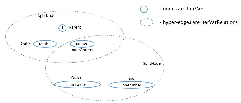
In the above example, the stage has one root_iter_var, i. It has been split, and the resulting inner axis i.inner, has been split again. The leaf_iter_vars of the stage are i.outer, i.inner.outer, and i.inner.inner.
Message passing functions are named “PassUp” or “PassDown”, depending on whether messages are passed from inner/outer IterVars to their parent (“PassUp”), or from the parent to the inner/outer children (“PassDown”).
InferRootBound
As mentioned in the previous section, the purpose of InferRootBound is to set the Range of each root_iter_var of the Stage’s operation. InferRootBound does not set the Range of any other IterVar, only those belonging to root_iter_vars.
If the stage is an output stage or placeholder, InferRootBound simply sets the root_iter_var Ranges to their default values. The default Range for a root_iter_var is taken from the ‘dom’ member of the IterVar (see the IterVarNode class declaration above).
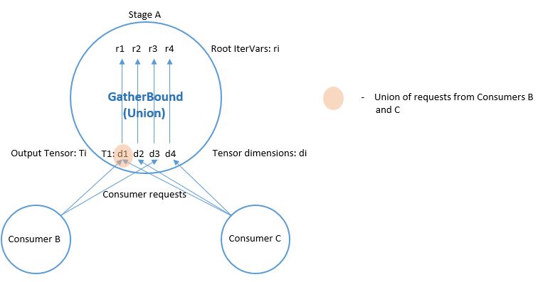
Otherwise, InferRootBound iterates through the consumers of the stage. IntSets are created for each of the consumer’s IterVars, as follows. Phase 1) IntSets are initialized for the consumer’s leaf_iter_vars, and propagated to the consumer’s root_iter_vars by PassUpDomain (Phase 2). These IntSets are used to create TensorDom of the output tensors of the stage (Phase 3). Finally, once all of the consumers have been processed, InferRootBound calls GatherBound, to set the Ranges of the stage’s root_iter_vars, based on the TensorDoms (Phase 4).
This process can seem complicated. One reason is that a stage can have more than one consumer. Each consumer has different requirements, and these must somehow be consolidated. Similarly, the stage may output more than one tensor, and each consumer only uses a particular subset of these tensors. Furthermore, even if a consumer uses a particular tensor, it may not use all elements of the tensor.
As mentioned above, a consumer may only require a small number of elements from each tensor. The consumers can be thought of as making requests to the stage, for certain regions of its output tensors. The job of Phases 1-3 is to establish the regions of each output tensor that are required by each consumer.

IntSets
During InferRootBound, Ranges are converted to IntSets, and message passing is performed over IntSets. Therefore, it is important to understand the difference between Ranges and IntSets. The name ‘IntSet’ suggests it can represent an arbitrary set of integers, e.g., A = {-10, 0, 10, 12, 13}. This would certainly be more expressive than a Range, which only represents a set of contiguous integers, e.g., B = {10,11,12}.
However, in TVM IntSets come in only three varieties: IntervalSets, StrideSets, and ModularSets. IntervalSets, similarly to Ranges, only represent sets of contiguous integers. A StrideSet is defined by a base IntervalSet, a list of strides, and a list of extents. However, StrideSet is unused, and ModularSet is only used by the frontend.
Therefore, not all sets of integers can be represented by an IntSet in TVM. For example, set A in the example above can not be represented by an IntSet.
InferBound is more complicated for schedules that contain compute_at. Therefore, we first explain InferBound for schedules that do not contain compute_at.
Phase 1: Initialize IntSets for consumer’s leaf_iter_vars
Input: rmap: consumer IterVar -> Range
Output: up_state: consumer leaf -> IntSet
In Phase 1, IntSets for each of the consumer’s leaf_iter_vars are created, based on the Ranges of the leaf_iter_vars from rmap. Recall that the consumer has already been visited by InferBound, so all of its IterVars have known Ranges in rmap.
There are three cases:
- Extent of leaf var’s Range is 1. In this case, the up_state for the leaf is just a single point, equal to the Range’s min.
- No relaxation is needed. In this case, the up_state for the leaf is just a single point, defined by the leaf var itself.
- Relaxation is needed. In this case, the leaf’s Range is simply converted to an IntSet.
For simplicity, we assume the schedule does not contain thread axes. In this case, Case 2 is only relevant if the schedule contains compute_at. Please refer to the section on “InferBound with compute_at” below, for further explanation.
Phase 2: Propagate IntSets from consumer’s leaves to consumer’s roots
Input: up_state: consumer leaf -> IntSet
Output: dom_map: consumer root -> IntSet
Phase 2 begins by calling PassUpDomain, which visits the IterVarRelations of the consumer stage. In the case of a Split relation, PassUpDomain sets the up_state of the parent IterVar, based on the inner and outer IntSets, as follows:
- Case 1: The Ranges of outer and inner IterVars match their up_state domains. In this case, set the parent’s up_state by simply converting the parent’s Range to an IntSet.
- Otherwise, the parent’s up_state is defined by evaluating outer*f + inner + (parent Range’s min), with respect to the up_states of outer and inner. Here, instead of using the Split relation’s factor, TVM uses f = extent of the inner IterVar’s Range.
Case 2 is only needed if the schedule contains compute_at. Please refer to the section “InferBound with compute_at” below, for further explanation.
After PassUpDomain has finished propagating up_state to all IterVars of the consumer, a fresh map, from root_iter_vars to IntSet, is created. If the schedule does not contain compute_at, the IntSet for root IterVar iv is created by the following code:
dom_map[iv->var.get()] = IntSet::range(up_state.at(iv).cover_range(iv->dom));
Note that if the schedule does not contain compute_at, Phases 1-2 are actually unnecessary. dom_map can be built directly from the known Ranges in rmap. Ranges simply need to be converted to IntSets, which involves no loss of information.
Phase 3: Propagate IntSets to consumer’s input tensors
Input: dom_map: consumer root -> IntSet
Output: tmap: output tensor -> vector<vector<IntSet> >
Note that the consumer’s input tensors are output tensors of the stage InferBound is working on. So by establishing information about the consumer’s input tensors, we actually obtain information about the stage’s output tensors too: the consumers require certain regions of these tensors to be computed. This information can then be propagated through the rest of the stage, eventually obtaining Ranges for the stage’s root_iter_vars by the end of Phase 4.
The output of Phase 3 is tmap, which is a map containing all of the stage’s output tensors. Recall that a Tensor is multi-dimensional, with a number of different axes. For each output tensor, and each of that tensor’s axes, tmap contains a list of IntSets. Each IntSet in the list is a request from a different consumer.
Phase 3 is accomplished by calling PropBoundToInputs on the consumer. PropBoundToInputs adds IntSets to tmap’s lists, for all input Tensors of the consumer.
The exact behavior of PropBoundToInputs depends on the type of the consumer’s operation: ComputeOp, TensorComputeOp, PlaceholderOp, ExternOp, etc. Consider the case of TensorComputeOp. A TensorComputeOp already has a Region for each of its Tensor inputs, defining the slice of the tensor that the operation depends on. For each input tensor i, and dimension j, a request is added to tmap, based on the corresponding dimension in the Region:
for (size_t j = 0; j < t.ndim(); ++j) {
	// i selects the Tensor t
	tmap[i][j].push_back(EvalSet(region[j], dom_map));
}
Phase 4: Consolidate across all consumers
Input: tmap: output tensor -> vector<vector<IntSet> >
Output: rmap is populated for all of stage's root_iter_vars
Phase 4 is performed by GatherBound, whose behavior depends on the type of operation of the stage. We discuss the ComputeOp case only, but TensorComputeOp is the same.
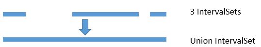
A ComputeOp has only a single output Tensor, whose axes correspond to the axis variables of the ComputeOp. The root_iter_vars of a ComputeOp include these axis variables, as well as the reduce_axis variables. If the root IterVar is an axis var, it corresponds to one of the axes of the output Tensor. GatherBound sets the Range of such a root IterVar to the union of all IntSets (i.e., union of all consumer requests) for the corresponding axis of the tensor. If the root IterVar is a reduce_axis, its Range is just set to its default (i.e., the ‘dom’ member of IterVarNode).
// 'output' selects the output tensor
// i is the dimension
rmap[axis[i]] = arith::Union(tmap[output][i]).cover_range(axis[i]->dom);
The union of IntSets is computed by converting each IntSet to an Interval, and then taking the minimum of all minimums, and the maximum of all of these interval’s maximums.
This clearly results in some unnecessary computation, i.e., tensor elements will be computed that are never used.
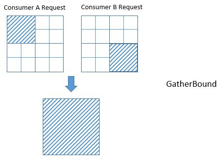
Unfortunately, even if we’re lucky and the IntervalSet unions do not produce unnecessary computation, the fact that GatherBound considers each dimension of the tensor separately can also cause unnecessary computation. For example, in the diagram below the two consumers A and B require disjoint regions of the 2D tensor: consumer A requires T[0:2, 0:2], and consumer B requires T[2:4, 2:4]. GatherBound operates on each dimension of the tensor separately. For the first dimension of the tensor, GatherBound takes the union of intervals 0:2 and 2:4, producing 0:4 (note that no approximation was required here). Similarly for the second dimension of the tensor. Therefore, the dimension-wise union of these two requests is T[0:4, 0:4]. So GatherBound will cause all 16 elements of tensor T to be computed, even though only half of those elements will ever be used.
PassDownDomain
The purpose of PassDownDomain is to take the Ranges produced by InferRootBound for the root_iter_vars, and set the Ranges of all other IterVars in the stage.
PassDownDomain iterates through the stage’s IterVarRelations (are they visited in any particular order?). There are three possible types of IterVarRelation: split, fuse, and rebase. The most interesting case, which offers opportunity for improvement, is IterVarRelations representing splits.
The Ranges of the inner and outer IterVars of the split are set based on the parent IterVar’s known Range, as follows:
- Range(inner): min = 0, extent = the split’s factor
- Range(outer): min = 0, extent = ceil(parent’s extent/factor)
There is an opportunity here to tighten the bounds produced by InferBound, when factor does not evenly divide the parent’s Range. Suppose the parent’s Range is 20, and the factor is 16. Then on the second iteration of the outer loop, the inner loop only needs to perform 4 iterations, not 16. If PassDownDomain could set the extent of the inner IterVar to min(factor, parent’s extent - outer*factor), then the extent of the inner variable would properly adapt, based on which iteration of the outer loop is being executed.
For Fuse relations, the Range of the fused IterVar is set based on the known Ranges of the inner and outer IterVars, as follows:
- Range(fused): min = 0, extent = (outer’s extent) * (inner’s extent)
For Rebase relations, which represent compute_at’s, the Range of the rebased IterVar is set based on the known Range of the parent IterVar, as follows:
- Range(rebased): min = 0, extent = parent’s extent
InferBound with compute_at
If the schedule contains compute_at, Phases 1-2 of InferRootBound become more complex.
Motivation
Ex. 1
Consider the following snippet of a TVM program:
C = tvm.compute((5, 16), lambda i, j : tvm.const(5), name='C')
D = tvm.compute((5, 16), lambda i, j : C[i, j]*2, name='D')
This produces the following (simplified IR):
for i 0, 5
    for j 0, 16
        C[i, j] = 5
for i 0, 5
    for j 0, 16
        D[i, j] = C[i, j]*2
It’s easy to see that stage D requires all (5,16) elements of C to be computed.
Ex. 2
However, suppose C is computed at axis j of D:
s = create_schedule(D.op)
s[C].compute_at(s[D], D.op.axis[1])
Then only a single element of C is needed at a time:
for i 0, 5
    for j 0, 16
        C[i, j] = 5
        D[i, j] = C[i, j]*2
Ex. 3
Similarly, if C is computed at axis i of D, only a vector of 16 elements of C are needed at a time:
for i 0, 5
    for j 0, 16
        C[i, j] = 5
    for j 0, 16
        D[i, j] = C[i, j]*2
Based on the above examples, it is clear that InferBound should give different answers for stage C depending on where in its consumer D it is “attached”.
Attach Paths
If stage C is computed at axis j of stage D, we say that C is attached to axis j of stage D. This is reflected in the Stage object by setting the following three member variables:
class StageNode : public Node {
public:
    // ommitted

    // For compute_at, attach_type = kScope
    AttachType attach_type;

    // For compute_at, this is the axis
    // passed to compute_at, e.g., D.op.axis[1]
    IterVar attach_ivar;

    // The stage passed to compute_at, e.g., D
    Stage attach_stage;

    // ommitted
};
Consider the above examples again. In order for InferBound to determine how many elements of C must be computed, it is important to know whether the computation of C occurs within the scope of a leaf variable of D, or above that scope. For example, in Ex. 1, the computation of C occurs above the scopes of all of D’s leaf variables. In Ex. 2, the computation of C occurs within the scope of all of D’s leaf variables. In Ex. 3, C occurs within the scope of D’s i, but above the scope of D’s j.
CreateAttachPath is responsible for figuring out which scopes contain a stage C. These scopes are ordered from innermost scope to outermost. Thus for each stage CreateAttachPath produces an “attach path”, which lists the scopes containing the stage, from innermost to outermost scope. In Ex. 1, the attach path of C is empty. In Ex. 2, the attach path of C contains {j, i}. In Ex. 3, the attach path of C is {i}.
The following example clarifies the concept of an attach path, for a more complicated case.
Ex. 4
C = tvm.compute((5, 16), lambda i, j : tvm.const(5), name='C')
D = tvm.compute((4, 5, 16), lambda di, dj, dk : C[dj, dk]*2, name='D')
s = tvm.create_schedule(D.op)
s[C].compute_at(s[D], D.op.axis[2])
Here is the IR after ScheduleOps:
// attr [compute(D, 0x2c070b0)] realize_scope = ""
realize D([0, 4], [0, 5], [0, 16]) {
  produce D {
    for (di, 0, 4) {
      for (dj, 0, 5) {
        for (dk, 0, 16) {
          // attr [compute(C, 0x2c29990)] realize_scope = ""
          realize C([dj, 1], [dk, 1]) {
            produce C {
              for (i, 0, 1) {
                for (j, 0, 1) {
                  C((i + dj), (j + dk)) =5
                }
              }
            }
            D(di, dj, dk) =(C(dj, dk)*2)
          }
        }
      }
    }
  }
}
In this case, the attach path of C is {dk, dj, di}. Note that C does not use di, but di still appears in C’s attach path.
Ex. 5
Compute_at is commonly applied after splitting, but this can be handled very naturally given the above definitions. In the example below, the attachment point of C is j_inner of D. The attach path of C is {j_inner, j_outer, i}.
C = tvm.compute((5, 16), lambda i, j : tvm.const(5), name='C')
D = tvm.compute((5, 16), lambda i, j : C[i, j]*2, name='D')
s = tvm.create_schedule(D.op)
d_o, d_i = s[D].split(D.op.axis[1], factor=8)
s[C].compute_at(s[D], d_i)
The IR in this case looks like:
for i 0, 5
    for j_outer 0, 2
        for j_inner 0, 8
            C[i, j_outer*8 + j_inner] = 5
            D[i, j_outer*8 + j_inner] = C[i, j_outer*8 + j_inner]*2
Building an Attach Path
The CreateAttachPath algorithm builds the attach path of a stage C as follows. If C does not have attach_type kScope, then C has no attachment, and C’s attach path is empty. Otherwise, C is attached at attach_stage=D. We iterate through D’s leaf variables in top-down order. All leaf variables starting from C.stage_ivar and lower are added to C’s attach path. Then, if D is also attached somewhere, e.g., to stage E, the process is repeated for E’s leaves. Thus CreateAttachPath continues to add variables to C’s attach path until a stage with no attachment is encountered.
In the example below, C is attached at D, and D is attached at E.
C = tvm.compute((5, 16), lambda i, j : tvm.const(5), name='C')
D = tvm.compute((5, 16), lambda di, dj : C[di, dj]*2, name='D')
E = tvm.compute((5, 16), lambda ei, ej : D[ei, ej]*4, name='E')
s = tvm.create_schedule(E.op)
s[C].compute_at(s[D], D.op.axis[1])
s[D].compute_at(s[E], E.op.axis[1])
The attach path of C is {dj, di, ej, ei}, and the attach path of D is {ej, ei}:
for ei 0 5
    for ej 0 16
        for di 0 1
            for dj 0 1
                for i 0 1
                    for j 0 1
                        C[i + ei, j + ej] = 5
                D[di + ei, dj + ej] = C[di + ei, dj + ej]*2
        E[ei, ej] = D[ei, ej]*4
InferBound with compute_at
Now that the concept of an attach path has been introduced, we return to how InferBound differs if the schedule contains compute_at. The only difference is in InferRootBound, Phases 1-2.
In InferRootBound, the goal is to determine Ranges for the root_iter_vars of a particular stage, C. Phases 1-2 of InferRootBound assign IntSets to the leaf IterVars of C’s consumers, and then propagate those IntSets up to the consumers’ root_iter_vars.
If there are no attachments, the Ranges already computed for the consumer’s variables define how much of C is needed by the consumer. However, if the stage is actually inside the scope of one of the consumer’s variables j, then only a single point from within the Range of j is needed at a time.
Phase 1: Initialize IntSets for consumer’s leaf_iter_vars
Input: rmap: consumer IterVar -> Range
Output: up_state: consumer leaf -> IntSet
In Phase 1, IntSets for each of the consumer’s leaf_iter_vars are created, based on the Ranges of the leaf_iter_vars from rmap. Recall that the consumer has already been visited by InferBound, so all of its IterVars have known Ranges in rmap.
There are three cases:
- Extent of leaf var’s Range is 1. In this case, the up_state for the leaf is just a single point, equal to the Range’s min.
- No relaxation is needed. In this case, the up_state for the leaf is just a single point, defined by the leaf var itself.
- Relaxation is needed. In this case, the leaf’s Range is simply converted to an IntSet.
Case 2 occurs if we encounter the attachment point of stage C in the consumer. For this attach_ivar, and all higher leaf variables of the consumer, Case 2 will be applied. This ensures that only a single point within the Range of the leaf variable will be requested, if C is inside the leaf variable’s scope.
Phase 2: Propagate IntSets from consumer’s leaves to consumer’s roots
Input: up_state: consumer leaf -> IntSet
Output: dom_map: consumer root -> IntSet
Phase 2 begins by calling PassUpDomain, which visits the IterVarRelations of the consumer stage. In the case of a Split relation, PassUpDomain sets the up_state of the parent IterVar, based on the inner and outer IntSets, as follows:
- Case 1: The Ranges of outer and inner IterVars match their up_state domains. In this case, set the parent’s up_state by simply converting the parent’s Range to an IntSet.
- Otherwise, the parent’s up_state is defined by evaluating outer*f + inner + (parent Range’s min), with respect to the up_states of outer and inner. Here, instead of using the Split relation’s factor, TVM uses f = extent of the inner IterVar’s Range.
Now, because the schedule contains compute_at, it is possible for Case 2 to apply. This is because the leaf IntSets may now be initialized to a single point within their Range (Case 2 of Phase 1), so the IntSets will no longer always match the Ranges.
After PassUpDomain has finished propagating up_state to all IterVars of the consumer, a fresh map, from root_iter_vars to IntSet, is created. If the stage is not attached to the current consumer, then for each variable iv in the consumer’s attach_path, iv’s Range is added to a relax_set. The root variables of the stage are evaluated wrt this relax_set.
This is to handle cases like the following example, where C is not attached anywhere, but its consumer D is attached in stage E. In this case, D’s attach_path, {ej, ei} must be considered when determining how much of C must be computed.
for i 0 5
    for j 0 16
        C[i, j] = 5
for ei 0 5
    for ej 0 16
        D[ei, ej] = C[ei, ej]*2
        E[ei, ej] = D[ei, ej] + 4